Using a VFD IV-3A tube to build a simple counter – Part four

Introduction

In part three the rest of the counter is build, and the circuit is almost complete. The part which is missing, is the thing that makes it count. We  could simply add a 4 bits binary counter, but why not simulate a counter ?

The HP8175A

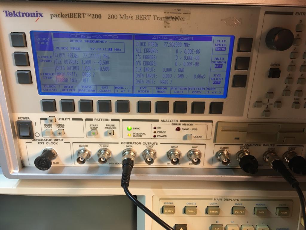
To simulate a simple 4 bits counter, I’m going to use my HP8175A. It’s big, it’s heavy, makes a lot of noise and eats a gazillion electrons per microseconds, and spits them out as heat. So what is not to love about this machine?

The interface of the HP8175A may take some time to get used at, but I loved it from the start. However to make it more interesting the HP8175A is programmed completely by IEEE-488. or GP-IB or a HP-IB  If you own a HP8175A and don’t have the possibility to remote control the machine, then study the user manual. It’s really not that difficult to program the HP8175A through the keyboard and knobs.

I used a National Instrument USB GPIB HS adapter to remote control the HP.

Remote control the HP8175A

To program the HP8175A a couple of steps must be taken. The HP8175A has so called “Module pages”. We need to:

    1. Setup on the Data Module the format: by setting up the POD and the duration.
    2. Setup on the Data Page the labels and bits which makes up the program
    3. Setup on the Program Page the program, the start end end labels, as well the times to run the program
    4. Setup the Clock page,
    5. And finally update all the settings and start the program

The IEEE-488 commands for the HP8175A is a bit cryptic, but this is the whole program:

RST
DM0;DUR0,1s;IFM(CLOCK),,,1111
DM1;CFM(CLOCK);TSA0;CHD0,(CLOCK),0000,0001,0010,0011,0100,0101,0110,0111,1000,1001;TSA9;CHD0,(END)
PM0;CD;(PROG1);CR7;CE;(END)
OM;POD 1
CM 0;CYM 1
UP;SA
LO

Explanation of the program

The commands and parameters are separated by a ‘;’. So for example the second line contains 3 commands: DM0 and DUR0 and IFM (Data Module, Duration Fixed, and Insert ForMat label)

    1. Reset HP8175A to defaults
    2. Go to page: Data Module FORMAT and set DUration to fixed 1 second and Insert ForMat label CLOCK and enable the first 4 POD lines (bits) of POD0
    3. Go to DATA page module and ChangeForMat label to CLOCK and Set
    4. ToStartAdress; CHangeData 0, CLOCK end set bits up to address 9 and change label to END ()
    5. Go to Program Module page and set the label PROG1, Move Cursor Right 7  positions, clear the field and change field so it contains the END label
    6.  Go to Output Module page and set all PODS enable
    7.  Goto Clock Module page and Set Clock to Auto Cycle
    8.  Update and start
    9.  Return to local (stop remote control, and enable front panel)

Line 3 might require some explanation:

DM1;CFM(CLOCK);TSA0;CHD0,(CLOCK),0000,0001,0010,0011,0100,0101,0110,0111,1000,1001;TSA9;CHD0,(END)

The part:

 TSA0;CHD0,(CLOCK),0000,0001,0010,0011,0100,0101,0110,0111,1000,1001

is quite clever. The engineers at the time by HP really know how to implement this kind of stuff. The command TSA needs a start address, which is the 0. Next command changes the format label to “CLOCK”. And then comes the clever part.

Since we enabled only for outputs on POD 0, we can have 4 bits on each address line. So by placing the 4 bits separated by comma’s, each bit pattern is placed on a address line. And therefore, this command places each 4 bits starting from address 0000 to 1001 (0 – 9).

So it works like:

                 4bits  4bits                                4bits
Set start addr   addr 0 addr 1                               addr 9
/|\               /|\   /|\                                   /|\
 |                 |     |                                     | 
TSA0;CHD0,(CLOCK),0000,0001,0010,0011,0100,0101,0110,0111,1000,1001

DECIMAL              0,   1,   2,   3,   4,   5,   6,   7,   8,   9

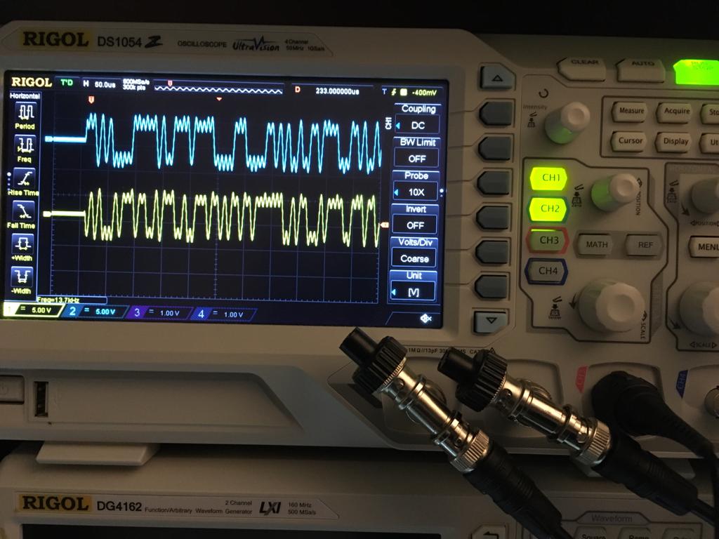
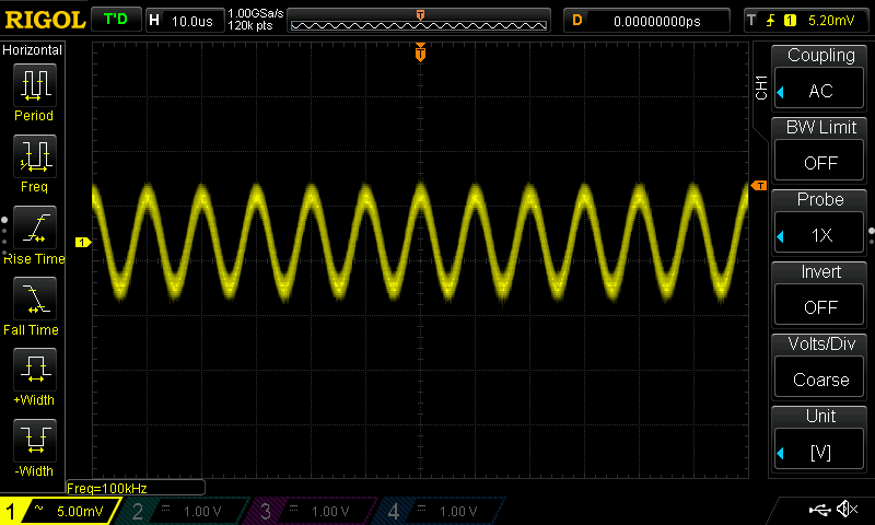
Let’s see the HP8175A in action

After sending the commands, the HP8175A is acting like a 4 bit binary counter:

Once I know the program is working I wrote a little pyton script using pyvisa:

import pyvisa
import time

# Small programm to remote control a HP8175A
# Using PyVisa with a NI USB GPIB-HS+

# Setup the resource manager
rm = pyvisa.ResourceManager()

#print(rm.list_resources())
# Open HP8175A
hp8175a = rm.open_resource('GPIB0::8::INSTR')

# Identify yourself!
print(hp8175a.query('IDN?'))
print(hp8175a.write('RST'))
time.sleep(5)

print(hp8175a.write('RST'))
print(hp8175a.write('DM0;DUR0,1s;IFM(CLOCK),,,1111'))
print(hp8175a.write('DM1;CFM(CLOCK);TSA0;CHD0,(CLOCK),0000,0001,0010,0011,0100,0101,0110,0111,1000,1001;TSA9;CHD0,(END)'))
print(hp8175a.write('PM0;CD;(PROG1);CR7;CE;(END)'))
print(hp8175a.write('OM;POD 1'))
print(hp8175a.write('CM 0;CYM 1'))
print(hp8175a.write('UP;SA'))
print(hp8175a.write('LO'))

Connecting a Rohde Schwarz AMIQ to a SMIQ04

Connecting a Rohde Schwarz AMIQ to a SMIQ04

The first article explains how to setup an R&S AMIQ and talk to it, and to get signals out of the I and Q outputs. In this article the AMIQ is connected to a SMIQ04. In this setup the AMIQ provides the IQ modulation, and the SMIQ is providing modulated signal on its RF output.

Prerequisites

To be able to use the SMIQ and AMIQ together, a vector modulator (IQMOD variant 4 or higher (var. 8) must be installed in the SMIQ.

Connecting the R&S AMIQ to R&S SMIQ

There are a couple of options on how to connect and control the R&S AMIQ. It’s possible to control the AMIQ from the SMIQ. Or control the AMIQ by a PC.In this setup I’m connecting the R&S SMIQ and R&S AMIQ together by the use of an IEEE-488 cable, so GPIB can be used to control the instruments.

One think to keep in mind is that when using the SMIQ to control the AMIQ, the SMIQ is acting as a controller. And there can only be one controller active on the bus at the same time.

The output “I” and”Q” of the R&S AMIQ must be connected to the “I” and “Q” inputs on tthe R&S SMIQ.

Generating signals

When using the SMIQ as a controller, the signals of the AMIQ can be used as follows:

In the menu Utilities/Install the option AMIQ control must be enabled. After enabling the SMIQ must be rebooted.

After reboot an extra menu option: IMQ CTRL is visible. In this menu the following options must be selected and set:

    • Start by setting carrier frequncy
    • Set the level of the output signal (for example 0 dBm)
    • Select the option: SELECT WAVEFORM
    • Next select: Drive and choose C:
    • Pick a waveform, or change to directory to select a waveform
    • Press return and select menu Mode.
    • In the Mode menu select AUTO
    • Press Return key, and select menu option Level
    • In the Level menu set the I and Q outputs to 0.5V/50 Ohm
    • Press return key, and go to Vector mod, and set state to “On”

The modulated signal should now be present on the RF output.

To demonstrate a modulated signal which is generated by the AMIQ I use a directional coupler.


I connected the directional couple’s input port the the RF output port of the SMIQ. The output port of the directional coupler is connected to a Tektronix 2225 scope. The CPL port is connected to a HP8591A.

Note that I connected the NOT I port, so I could create a interesting signal, which is a challenge to trigger on the Tek 2225.


Getting an Rohde Schwarz AMIQ up and running

Introduction

The Rohden Schwarz AMIQ is an IQ modulation generator. According to the documentation of Rohden Schwarz this device has:


    • 100 MHz sample rate
    • 16 M Samples memory depth
    • IF generation up to 25 MHz
    • Multiple carrier simulation

And the best part is.. these devices can be picked up for little money.  Even if one is not into IQ modulation and such, the device is able to put out some very nice looking sine waves. There is a catch however. (There is always a catch): The AMIQ can only be controlled remotely.

What to look for when buying an AMIQ

When buying an AMIQ, look at the options the unit has. The user manual which can be found online, list all the available hard-, and software options.

Secondly, the AMIQ has a built in hard disk. If this drive is damaged, you could be out of luck. I searched online, but could not find any firmware images. If you bought an AMIQ, then make a image of the internal hard disk.  The AMIQ boots OpenDos.

There is an easy way to determine if the AMIQ is in a working condition. And that is to listen to the beeps at startup. The device will give one beep when turned on, and a few moments later, a second beep is produced. It’s the AMIQ’s way of letting you know it’s past it’s error checking thing. This second beep,should be followed by a steady green LED on the front panel.

If none of the above is happening, the AMIQ is having a fault, or the AMIQ didn’t start in a sane state. There seems to be a service manual for the AMIQ, where you can troubleshoot. Unfortunately I could not find the service manual online.

So when buying an AMIQ, let the seller boot up the AMIQ, and let the seller describe to you the boot process.

Once you got physical access to the AMIQ, you could run the the command:

*TST?

This should return a 0 when no errors are found, or a 1 if a error is found. The user manual describes in detail how to hardware test the AMIQ. Also note that the above command doesn’t test the RAM memory.

The third thing you may be aware of, are the different models:

    • AMIQ02
    • AMIQ03
    • AMIQ04

I never encounter the AMIQ01, however the AMIQ03 and 04 are the newer models, with more memory, sample rates etc. The main difference between the AMIQ03 and 04 is greater memory: The 04 has up to 16 000 000 IQ values, compared to the 03: 4 000 000 I/Q values)

Only the models 03 and 04 can have the option “AMIQ-B3” fitted. So if you see an AMIQ listed with the option “AMIQ-B3” you know it has to be a 03 or 04 model.

Controlling the AMIQ

To let the AMIQ do something useful, like spitting out signals, the AMIQ needs remote control. And for this remote controlling there are several options:

    • Through serial connection
    • Through IEEE-488 (GP-IB or also called HP-IB)
    • Use an Rohde Schwarz SMIQ
    • Use software like WinIQSim (version 1.x)

Luckily I got all the options…

Talking to the AMIQ

The easiest way of getting the AMIQ up and running is to connect a null modem cable to the RS232 port. If someone has changed the default serial parameters (9600,8n1) an formatted floppy disk (MSDOS) is needed with the file: AUTOEXEC.IEC with the following line:

:SYST:COMM:SER:BAUD 9600

Insert the floppy disk into the AMIQ, turn the AMIQ off, and on again. Once the AMIQ is fully booted, the serial console should be accessible.

When you have the luxury of having IEEE-488 or you could reset the the default address 6 with similar procedure, the line in the AUTOEXEC.IEC must be:

:SYST:COMM:GPIB:ADDR 6

Once a working connection is established to the AMIQ, the following command should give you the directories on the hard drive C:

:MMEM:DIR?

To load an waveform, and put out the signals on the I and Q outputs, give the following commands:

*RST;*CLS;*WAI
:MMEM:CD 'C:\'
:MMEM:LOAD RAM, 'GSM_TSC1.WV,TRAC'
:TRIG:MODE CONT
:OUTPUT:I FIX
:OUTPUT:Q FIX

The commands on the first line resets the device. Next the directory is changed to the C: drive. On the third line a waveform called: “GSM_TSC1.WV” is loaded into RAM memory. By setting the trigger to continuous on the next line, the waveform is send to the outputs, which are enabled on the last two lines.

This produces the following signal:

In the next article I’m going to hook up the AMIQ to the Rohde and Schwarz SMIQ04 and generate some signals.

Using a VFD IV-3A tube to build a simple counter – Part three

Introduction

In part two an ULN2023 is used so we can connect the IV-3A segments to 20V, while driving the segment with 5V. In this part the IV-3A is connected to the ULN2803A, and a 74LS48 which is BCD to 7-Segment Decoder.  By using the 74LS48 we can use 4 bits to drive the 7 segments.

Connecting the IV-3A

To connect the IV-3A to the IV-3A follow the following table:

IV-3A connections

IV-3A ULN2308
5 8
6 7
10 6
1 5
2 4
3 3
4 2

The last connections to make are the grid and heater. The schematic looks like:

IV-3A connections
IV-3A connections

Connect the 74LS48

The datasheet for the 74LS48 can be found here. Before connecting up the 74LS48, we need to invert the signals. Since the ULN2308 is a NPN Darlington array, we  need to invert the signals, so that a segment is activate when the input signal is going HIGH, instead of LOW.

An easy solution is to use a HEX invert. Since a HEX invert, as the name implies has 6 inverters, so we need two of them. So 2x a 74LS04 is going to be used.

The schematic looks like:

Display Driver schematic

When connecting the all the BCD (248) inputs( pins: 76,2,1) to GND, the IV-3A should show a “zero”.   Like wise, if we connect these pins to 5V, a 8 is shown. The table below show the BCD coding for the pins:

BCD (248) conversion table

A3 A2 A1 A0 Digit
0 0 0 0 0
0 0 0 1 1
0 0 1 0 2
0 0 1 1 3
0 1 0 0 4
0 1 0 1 5
0 1 1 0 6
0 1 1 1 7
1 0 0 0 8
1 0 0 1 9

In the next article the HP8175A is going to be used as a binary 4 bits counter.

Using a VFD IV-3A tube to build a simple counter – Part two

Introduction

In the first part I mentioned that I used 2 DC-to-DC converters. In this article we’re going to see how these modules are connected, and a ULN2803A is used to connect the segments to 20V, while driving the segments from a 5V rail.

Connecting the DC-to-DC converters

The connection of the DC-to-DC converters is very simple:This simple schematic shows how the modules are connected to the 5V rail.

One the modules are connected, the voltages needs to be set. This is done by turning a potentiometer. The XL6009E1 is set to +/- 20V while the HX-mini-360 is set to 1V.

Connecting the ULN28023

The ULN28023 is a Darlington array. Here you can find the datasheet.

The datasheet mention the following description:

The ULN2803Adeviceis a 50 V, 500 mA Darlington transistor array.The device consists of eight NPN Darlington pairs that feature high-voltage output swith common-cathode clamp-diodes for switching inductive loads.The collector-current rating of each Darlingtonpair is 500 mA. The Darlington pairs maybe connected in parallel for higher current capability. Applications include relay drivers,hammer drivers,lamp drivers,display drivers(LED and gas discharge),line drivers,and logic buffers.The ULN2803A device has a 2.7-kΩ series base resistor for each Darlington pair for operation directly with TTL or 5-V CMOS devices

So this IC is perfect to drive the VFD tube. Connecting the ULN2803 is simple:

In The next article the VFD tube is connected, and a 74LS48 is used to drive the the tube.

How to create layer 2 trunk port and access vlans on a Juniper SRX

Introduction

Creating vlans on a Juniper SRX is not as straight forward if you’re used to Cisco gear for example. In this article I hope to explain how to create:

      • One port as a trunk port
      • Other ports as access port
      • Add a mgmt L3 interface

Creating the trunk port

Let’s first create the trunk port. The interface fe-0/0/0 is used as a uplink port to another switch, and this ports carriers multiple tagged vlans. And it carriers only tagged vlans. No untagged vlan is allowed on this port.

To configure the port as a trunk port, the  port-mode has to be set to “trunk” and the allowed vlans needs to be configured. In this case the tagged vlan id’s are: 100,102:

set interfaces fe-0/0/0 description UPLINK-BB-SLV-LAN-P1.0.12
set interfaces fe-0/0/0 unit 0 family ethernet-switching port-mode trunk
set interfaces fe-0/0/0 unit 0 family ethernet-switching vlan members vlan-102
set interfaces fe-0/0/0 unit 0 family ethernet-switching vlan members vlan-100

Note that the vlan names are used, which at this point still needs to be created. It’s also possible to specify the vlanid here:

set interfaces fe-0/0/0 description UPLINK-BB-SLV-LAN-P1.0.12
set interfaces fe-0/0/0 unit 0 family ethernet-switching port-mode trunk
set interfaces fe-0/0/0 unit 0 family ethernet-switching vlan members 102
set interfaces fe-0/0/0 unit 0 family ethernet-switching vlan members 100

Create the vlans

Creating the vlans is straightforward:

set vlans vlan-100 vlan-id 100
set vlans vlan-102 vlan-id 102

Create the access ports

Creating the access ports is just like creating a trunk port, accept the port-mode is set to .. yes you guessed it.. ‘access‘.  So let’s assume we want to set the ports fe0/0/01 – fe0/0/7 as access ports with vlan 102.

set interfaces fe-0/0/1 unit 0 family ethernet-switching port-mode access
set interfaces fe-0/0/1 unit 0 family ethernet-switching vlan members vlan-102
set interfaces fe-0/0/2 unit 0 family ethernet-switching port-mode access
set interfaces fe-0/0/2 unit 0 family ethernet-switching vlan members vlan-102
set interfaces fe-0/0/3 unit 0 family ethernet-switching port-mode access
set interfaces fe-0/0/3 unit 0 family ethernet-switching vlan members vlan-102
set interfaces fe-0/0/4 unit 0 family ethernet-switching port-mode access
set interfaces fe-0/0/4 unit 0 family ethernet-switching vlan members vlan-102
set interfaces fe-0/0/5 unit 0 family ethernet-switching port-mode access
set interfaces fe-0/0/5 unit 0 family ethernet-switching vlan members vlan-102
set interfaces fe-0/0/6 unit 0 family ethernet-switching port-mode access
set interfaces fe-0/0/6 unit 0 family ethernet-switching vlan members vlan-102
set interfaces fe-0/0/7 unit 0 family ethernet-switching port-mode access
set interfaces fe-0/0/7 unit 0 family ethernet-switching vlan members vlan-102

However, this is a lot of typing. With junos it’s possible to use an interface range configuration. This is somewhat different to Cisco’s IOS or IOS-XE.

To use a interface range, first create a interface range name. For example ‘access-ports’. Then the name ‘access-ports’ can be used to add members. Next the properties of the interfaces can be assigned.

This might sound complex, but it’s quite simple and easy to use (and powerful):

set interfaces interface-range access-ports member "fe-0/0/[1-7]"
set interfaces interface-range access-ports unit 0 family ethernet-switching port-mode access
set interfaces interface-range access-ports unit 0 family ethernet-switching vlan members vlan-102

Assign the interfaces to the vlans

In the last step, the interfaces needs to be assigned to the vlans. So to assign the trunk port and access port to vlan 102 we need to do the following:

set vlans vlan-102 interface fe-0/0/0.0
set vlans vlan-102 interface fe-0/0/1.0
set vlans vlan-102 interface fe-0/0/2.0
set vlans vlan-102 interface fe-0/0/3.0
set vlans vlan-102 interface fe-0/0/4.0
set vlans vlan-102 interface fe-0/0/5.0
set vlans vlan-102 interface fe-0/0/6.0
set vlans vlan-102 interface fe-0/0/7.0

Note: the interfaces added are added by using the unit number, which is 0 here.

The above could be done in one command: simply by using the previous defined interface range ‘access-port’:

set vlans vlan-102 interface access-ports

When the an interface range is used, the trunk ports needs to be added as well:

set vlans vlan-102 interface fe-0/0/0.0

At this point the configuration can be committed:

commit

At this point, the layer 2 configuration is complete. The most easiest way to check if everything works is to look at the mac table. The command to do this is:

show ethernet-switching mac-learning-log

If everything is well it’s shows the learned mac addresses.

Create a Layer 3 management interface

To manage the SRX, it might be handy to have management vlan. In this case vlan id 100 is used.

To add a layer 3 vlan interface the next configuration is needed:

First create the vlan interface:

set interfaces vlan unit 100 family inet address 10.90.0.14/24

Next the interface can be added to the vlan 100:

set vlans vlan-100 l3-interface vlan.100

To activate to configuration don’t forget to do a commit:

commit

Using a VFD IV-3A tube to build a simple counter

Introduction

Some time ago I figured out the pins of of IV-3A VFD tube. In the upcoming articles series I’m going to build a simple counter, and planning to use some of my LAB equipment to test and build this counter. Just for fun.

Roughly I’m thinking of planning the following articles :

      • Implement the PSU for the different voltages (1V,5V,20V)
      • Design and implement the display driver
      • Use the HP 8175A to simulate a 4 bit binary counter
      • Using a Hp8110A as a serial data generator to simulate a 4 bit counter
      • Finally build the counter

Implement the PSU for the different voltages (1V,5V,20V)

One of the first challenges when working with a VFD tube is getting all the different voltage rails required. The IV-3A tube needs the a couple of voltages: 1V,5V,20V

The get the 5V rail is not a real problem, 1V and 20V can be more difficult.

To start with the 1V rail, one might think of a simple voltage divider, but this is not as simple as it sounds. When trying to drive the heaters, this will add a load to the voltage diver. Which lowers the voltage, resulting in a voltage which is to low. This could be addressed by adding a opamp, as a buffer. However the circuit is going to get more and more complex.

So in this design I’m going to use small DC-to-DC converters. Or step-up converts to be more precise. And I use two modules:

      • One module to step up the voltage to 20v
      • One module to down convert the voltage to 1V

The modules ‘m going to use are:

      • XL6009E1
      • HX-mini-360

These modules are cheap, and easy to use.

The downside to this is that the heater could be driven “to hard”, on the other hand, these tubes can take somewhat of a “punishment”. I’ll keep the rest of  the voltages low by driving the tube with 20V instead of the max 30V.

Both of the DC-to-DC converter modules are driven from a 5V supply. This makes it easy to implement the modules.

In the next article the display driver is going to be implemented.


Testing max data throughput on a BreadBoard

Testing max data throughput on a BreadBoard

After I repaired the Tektronix Bert tester PB200 I can finally do a test which I wanted to do for a long time. And that is to test the max data throughput of a breadboard. So in other words: What is the max speed at which data can travel through a breadboard (BB) without any errors ?

I came up with two tests:

      • The first test is to use a couple of rows on the BB
      • The second test is to use a power rail

Preparing the first test

The test setup is quite easy, just a few wires on a bread board. I didn’t put the wires across the whole length of the BB, at that point a lot of other stuff comes into play. Just by adding a few wires I get (roughly) an idea what the impact of extra connections is.

And to get an initial impression I started the test with just connecting the probes to a BB and measure the data transfer. This gives me a base line of 80 Mhz.

Next I prepare the BB as follows:

As can be seen just a couple of connections to generate some contact resistance. The BB and wires will add some capacitance too.

The test results of the first test

This results in:

It’s somewhat hard to read from the reflecting screen, but the max throughput I got after running this test for a couple of hours is around 77Mhz. So compared to the earlier test, adding a couple of wires resulted in a loss of 11Mhz. Which is quite a loss.

But note that this is is quick test. I didn’t use a loaf of 50Ohms, and I used a good quality BB (BusBoard Prototype Systems BB830).

Setting up the second test

The second test looks like:

Once this is setup I ran the test. When a test fails it looks like:

When an error occurs I lower the frequency, and reset the error. And the end

Results of the second test

I could get a max throughput of:

So it’s very close to 80 Mhz. However in a real case scenario don’t expect to send data across with this high speeds. In reality I ques somewhere around 10 Mhz till 40Mhz is more realistic.

Having fun with a R&S SMT03 and HP8591A Spectrum Analyzer

Playing around with the R&S SMT03 and an HP8591A Spectrum Analyzer

Now that I fixed the R&S SMT03 I find finally time to play around with the SMT03. The idea is to learn more about modulation, and how to display this on a Spectrum Analyzer. In a previous article I used the Siglent SSA 3021X Spectrum Analyzer in this article I’m going to use a HP 8591A Spectrum Analyzer.

Preparing the R&S SMT03

First off I need to setup the R&S SMT03

I’m going to use a carrier signal of 100Khz, and AM dept of 27%. And since the SMT03 have a second LF Generator I use that one to generate a sinus wave of 1.000 Khz. To protect the input of the HP SA I set the amplitude to 0 dBm.

Setting up the HP8591A Spectrum Analyzer

After setting up the R&S SMT03 it’s time to configure the HP8591A

After setting the center frequency the SPAN is set to 20 Mhz. To see the AM modulation, a smaller SPAN is needed. After the SPAN is set to 1.5Mhz the AM modulation becomes visible:

This shows the AM modulation. I really like the HP 8591A SA, it has a easy to use interface. And having a R&S SMT03 and the HP8591A in my lab is really awesome.

Use a spectrum analyzer to find interfering signals

Understanding the difference between Oscilloscope and Spectrum Analyzer

Before diving into the use of a Spectrum Analyzer (SA), a short explanation between an Oscilloscope and a SA might be handy. If you used a SA before, this article might not be to any interest to you, since this article covers a basic understanding.

For those who a curious to what a SA is, hang around, since this article is about to demonstrate the difference between a  Oscilloscope ans a SA.

When starting with electronics, sooner or later you might find yourself wanting an Oscilloscope to look at (fast) changing electronic signals. In other words: An scope is a multi functional tool in a electronics lab, and every good electronics labs should have one. With a scope it’s possible to look at electronic signal, being it digital signal or analogue signal which changes over time. But a scope can also be used to measure voltages, and all other characteristics of a signal. For example, the fall and rise time of edges, period of a signal, the max and min voltages, and perform math functions on signals.

Using a Oscilloscope to look at a signal

Most often a scope is used to look at a signal, and see how it looks like. For example a sinus signal:

Looking at the signal we can tell that the signal is 50mV (Peek to Peek), and that the frequency of the signal is 100Khz. Looking at the signal closer, it’s not a sharp clean sinus signal. So what’s wrong ?

If we zoom into the signal to have a closer look, the signal looks like:

This is doesn’t look like a clean signal. At this point several things may be the cause:

      1. Is there something which interferes with the signal?
      2. Is the measurement done properly (aka signal integrity)

This is the point, where it’s very difficult, to use a scope to investigate this further. Just let’s assume that this is no measurement fault. Short ground leads are used, and the probes are calibrated.

That leaves us with a interfering signal of some kind.

      • How to determine what kind of signal this is?
      • What is the frequency of this interfering signal ?

At this point some want’s to use a feature which is called “FFT” which some  scope might have.  FFT stands for: Fast Fourier Transform spectrum analyser  When using this feature the scope is behaving like a SA.

Having a FFT feature on a scope might be handy, in my case the FFT feature on my Rigol Ds1054Z is not very helpful:

It shows that there seems to be an extra signal, but it’s not possible to get any detail on this signal. To get more detail, a real Spectrum Analyzer is needed.

What is a Spectrum Analyzer (SA)

A Spectrum Analyzer might at first glance be some kind of a scope. It has a display to show signals, and has a lot of buttons, like a scope.

However the main difference between a scope and SA is that:

      • A scope shows signals in the time domain
      • A SA shows signals in the frequency domain

This means that a SA show on the horizontal the frequency, and on the vertical the power of the signal, which is shown in  a Logarithmic scale. This can be for example in dB or dBm. The reason for displaying the power (on a scope you would say the amplitude) of the signal in a Logarithmic scale  is that low power signal can be displayed next to high power signals.

And since a SA displays signals in the frequency domain, it’s possible to see how “pure” or “clean” a signal is, since we can actually look at the “spectrum” of the signal. Hence why it’s called a “Spectrum Analyzer”.

Using a Spectrum Analyzer to look at a signal

Let us look at the same signal which we looked at on the scope, but now feed into a Spectrum Analyzer:

Here is the same signal, but it looks quite different from the signal which is shown on the scope. However it’s frequency is 100Khz, and the power of the signal is -46.00 dBbm. Which is about 3.169 mVpp (There is some loss in the cables, and adapters used).

Looking at the signal it’s seems “not clean”, But it’s hard to see. So like on a scope, it’s possible to zoom into the signal, and get more detail. To this we need to set a smaller SPAN. The SPAN on a SA is the bandwidth were we are looking at it. It’s like the zoom-lens on a camera, by zooming in, more details are visible. Currently the SPAN width is 20.000Khz.

If we change the SPAN width to let’s say 1.000Khz, we see the following:

And suddenly a second signal appeared. To get more details about this signal, the SA provides a easy way, and that’s by placing a marker. In this case a delta marker is used. A delta marker can show the difference (delta) between signals.

And then we see that the interfering signal is a 100Hz away from our original signal of 1oo.ooo Khz signal.  So the interfering signal is 100.1 Khz.

Conclusion

And this shows the difference between a scope and a SA. An SA is a very handy tool when looking at the spectrum of a signal. It’s how every a more complex, and sometimes more confusing tool to use. On the other hand, a scope is also a complex tool to use. But in general, a scope is much more used for looking at signal then a SA. A SA is mostly used when dealing with RF, radio’s transmitters and alike.